

End-to-End Data Pipeline Series: Tutorial 1 - Introduction

Welcome to the “End-to-End Data Pipeline” series!
This is the first post in a series where we’ll build an end-to-end data pipeline together from scratch.
Building a data pipeline can be a daunting task. There are so many tools and technologies to choose from, and it can be hard to know where to start.
In this series, we’ll begin with the basics and gradually build up to a full-fledged data pipeline using an example e-commerce dataset.
We’ll be using open-source tools for each part of the pipeline so you can follow along and build your own data pipeline.
Overview of What We’ll Be Building
Here’s what’s in store for this series:
- Introduction to End-to-End Data Pipeline (this post)
- Data Storage with MinIO/S3 and Apache Iceberg
- Data Ingestion with Meltano
- Data Transformation with DBT and Trino - Part 1
- Data Transformation with DBT and Trino - Part 2
- Data Orchestration with Dagster
- Data Visualization with Superset
- Building end-to-end data pipeline with Sidetrek
Before we get to the nitty-gritty of how to build the data pipeline, let’s take a step back and understand what a data pipeline is and how it works.
Keeping this big picture in mind will help us navigate the details throughout this series.
What is a data pipeline?
You can think of data as a flow. It is generated somewhere, changed, and then served to someone who will use that data to do something useful.
The data pipeline is how the data flows.
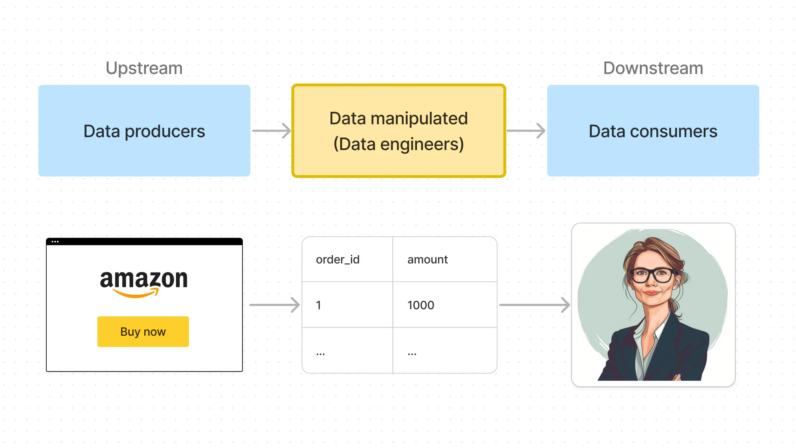
As seen in Figure 2, a simple example of this is when a visitor buys something on Amazon. When the visitor completes a checkout process, an “order” data is generated.
This is the “Generation” part of the data pipeline - the “data source” is the Amazon website tracking.
Then the data flows through the pipeline until it reaches the “data consumer” - maybe a Finance Manager who wants to know how much sales Amazon made last month.
The data pipeline is how data flows from data sources to data consumers. And the core job of data engineers is building and maintaining this pipeline.
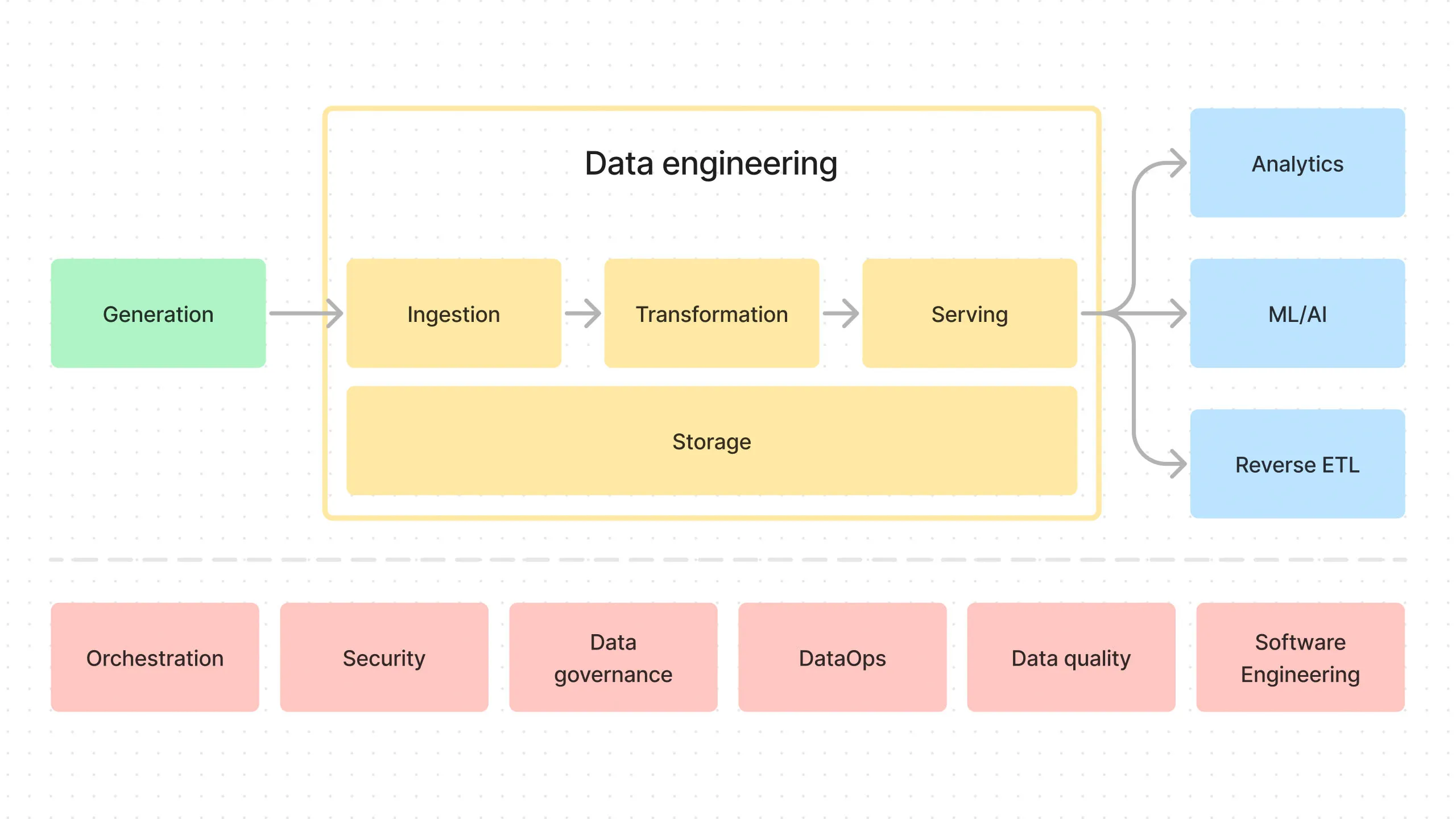
Generation
It all starts with “Generation” (the green box in Figure 1), where the data is originally generated.
This could be website tracking data, sales team data from Salesforce, databases, payments data from Stripe, sensor data, cloud logging data, etc.
Typically, data generation is outside of the control of data engineers.
This makes things challenging because unexpected data can enter the pipeline. It’s the job of the data engineers to ensure the pipeline is robust enough to handle changes in the incoming data.
Ingestion
The generated data is ingested into the data pipeline (the yellow “Ingestion” box in Figure 1).
This is the EL part of the commonly known ETL/ELT (Extract, Load, Transform). We’re extracting data from the data sources and loading it into our storage system.
The tricky part about ingestion is that we’re dealing with many third-party systems. Imagine the data generated by a website, a CRM system, a payments system, IoT devices, etc. Each of these systems has its own API, which we have to connect to and pull data from.
You have to build and maintain connections to each of these systems. This is where “managed connector” tools like Meltano come in.
We’ll see how to set up Meltano during the Ingestion part of the series.
Storage
The ingested data is stored in a storage system (the yellow “Storage” box in Figure 1). The storage system underpins the entire data pipeline since the data is ingested, transformed inside it, and then served from it.
This storage system is commonly a data warehouse like Snowflake or a data lakehouse like Apache Iceberg, which has been gaining popularity recently.
It’s critical to pick the right storage technology for the job.
There are many storage options, but we can broadly categorize them into two types: 1) row-based storage and 2) columnar storage.
Row-based storage is good for transactional data, where you’re reading and writing individual rows of data - for example, a single order from a user.
Columnar storage is good for analytical queries where you’re aggregating data across many rows - for example, total sales for the last month.
Using row-based storage like Postgres can incur a huge performance penalty when you’re running analytical queries on a large dataset. This is where columnar storage like Apache Iceberg comes in.
We’ll learn more about Apache Iceberg during the Storage part of the series.
Transformation
The ingested data is then transformed into a form more suitable for business analytics.
The transformation step can get quite complex if you have to join data from multiple sources, clean the data, aggregate it, etc.
To make this process easier, we use tools like DBT, which lets you write SQL queries to transform the data. Think of DBT as a supercharged SQL builder that lets you create complex data transformations in a modular way.
But DBT can’t actually execute the queries. For that, we need a query engine like Trino. Trino is a distributed SQL query engine that can run complex queries on large datasets.
We’ll see how to set up and connect DBT and Trino during the Transformation part of the series.
Serving
Finally, this transformed data is served to data consumers like business analysts, data scientists, etc.
At the end of this series, we’ll assume the role of a business analyst and see how we can visualize the data using Apache Superset.
Undercurrents
In Figure 1, you can see the dotted line separating the top and bottom parts of the diagram. The bottom part is “undercurrents” (I’m borrowing the term from the excellent book “Fundamentals of Data Engineering” by Joe Reis and Matt Housley).
The undercurrents underlie the entire data pipeline. Orchestration, security, DataOps, etc.
We’ll touch on some of these topics as we build the data pipeline, but one important one is orchestration.
An orchestrator like Airflow or Dagster is the conductor of the data pipeline. It schedules the tasks, monitors their progress, and handles any failures. Without it, the data pipeline would be very brittle.
We’ll be using Dagster as our orchestrator, so we’ll dig deeper into how we set up and use Dagster during the Orchestration part of the series.
Data Pipeline Architecture for This Series
So here’s how our end-to-end data pipeline will look by the end of this series:
- Minio (local replacement for S3) and Apache Iceberg for data storage
- Meltano for data ingestion
- DBT and Trino for data transformation
- Dagster for orchestration
- Superset for data visualization
Different Use Cases
There are many use cases for different data pipelines. Let’s take a look at some examples to see how data pipelines can be used for different scenarios.
Business Analytics (or Business Intelligence or BI)
The first one is the most common use case, which is business analytics.
PetCo manufactures and sells pet toys. It has a website that sells directly to consumers, generating customer and order data. It uses Stripe as a payment processor, generating payment data. It also has a sales team that sells to retail shops in bulk, using Salesforce as its CRM and generating wholesale sales data.
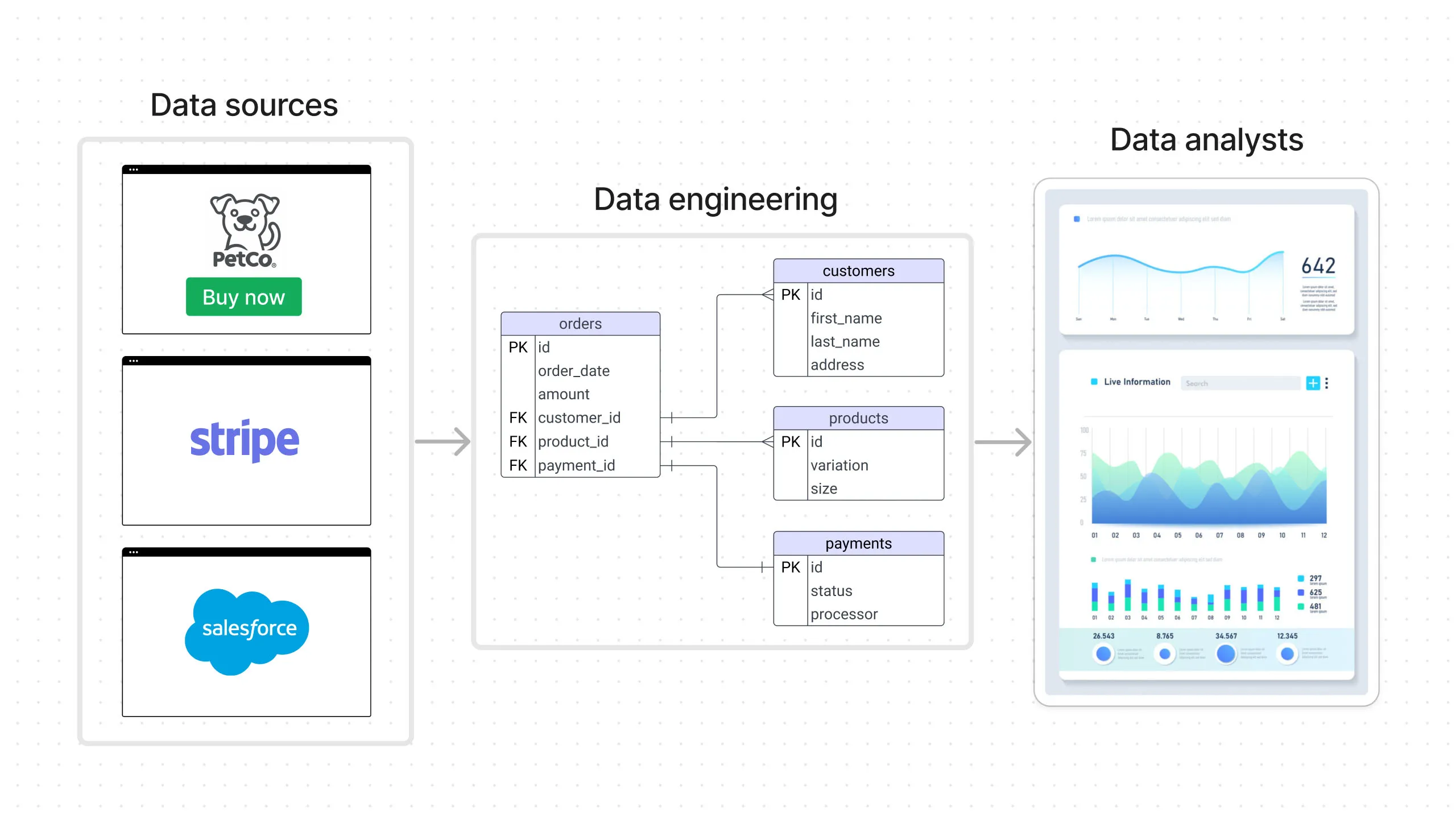
All this data is sent to the data engineering team, which aggregates all these data sources, stores it, and transforms it into a form that can be easily consumed by data consumers. Data consumers here can be business analysts who will create a dashboard of business performance to be used by the executives.
Real-time
Another example is a real-time use case for Doordash. A Doordash user orders dinner from her favorite restaurant. The delivery person picks up this order and starts sending updates, including whether they picked up the order and their current location using their phone’s GPS.
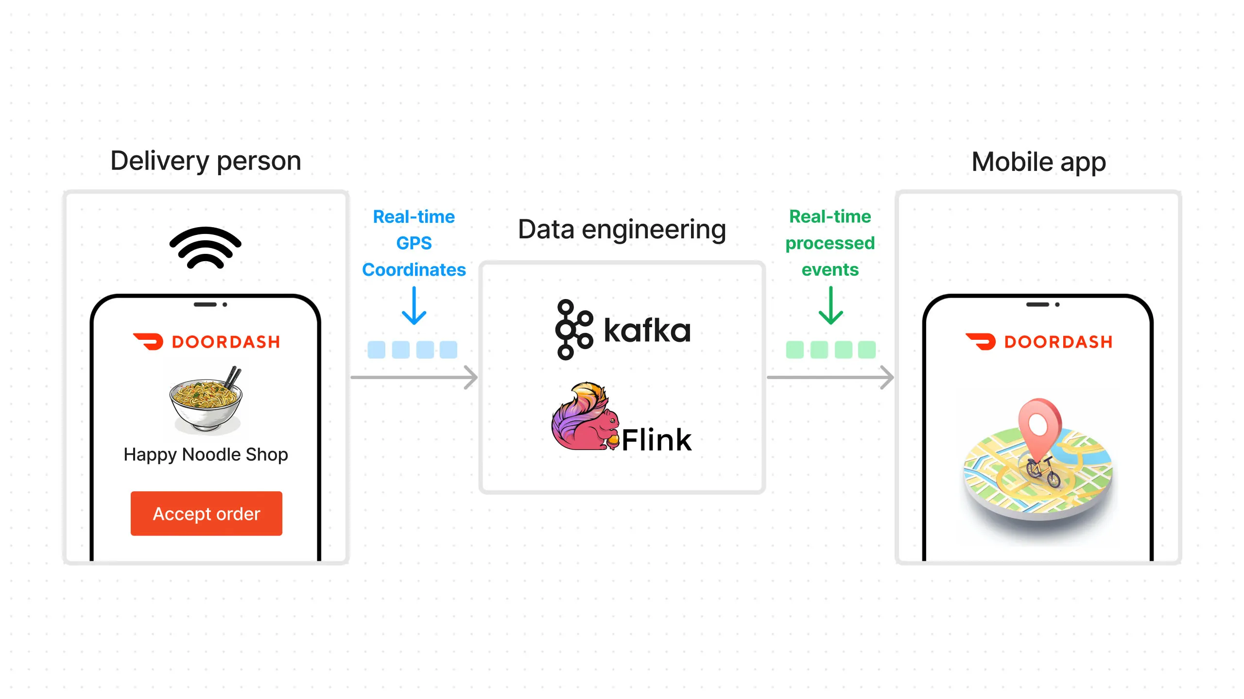
This data is sent in real-time to the data engineering team, which uses event streaming and processing systems like Kafka and Flink to process the data and send it over to our user’s Doordash app, which displays the delivery status. All this needs to happen in seconds end-to-end so the user knows what’s happening with their delivery at all times.
This might sound easy, but let’s put this into perspective. Doordash users create hundreds of billions of events and petabytes of data per day. Data engineers must build systems that can handle this massive amount of data and ensure millions of orders each day get real-time updates without fail.
ML
What about ML use cases? Unlike business analytics use cases, which work with historical data, ML use cases involve predicting the future.
Let’s use Instacart as an example. Instacart needs to predict if the items users order will be available in the grocery store. It’s the “likely out of stock” feature you see in their mobile app.
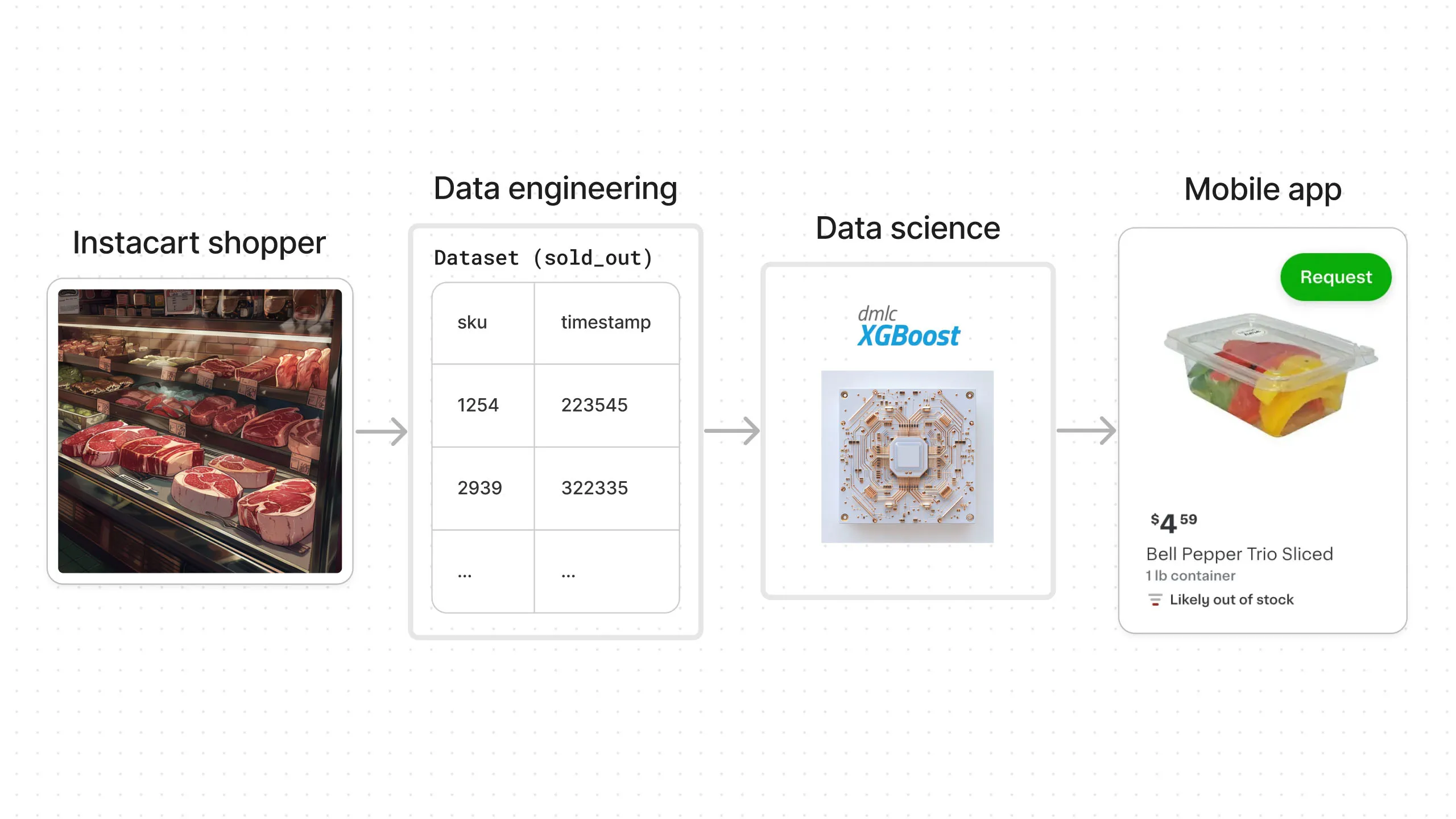
You might think this should be easy, but grocery stores don’t actually tell Instacart what items are available and what items are sold out, which makes this task surprisingly challenging.
The Instacart shopper sends information about which items are sold out and when, as they shop for customer orders. This information is then sent to the data engineering team. The data is collected over time, cleaned, and transformed into a dataset that is sent to the data science team.
Data scientists then build an ML model using this data, which is used to predict item availability. That’s the “likely out of stock” feature you see in Instacart’s mobile app.
AI
The final example we’ll look at is an AI use case — specifically, a deep learning use case.
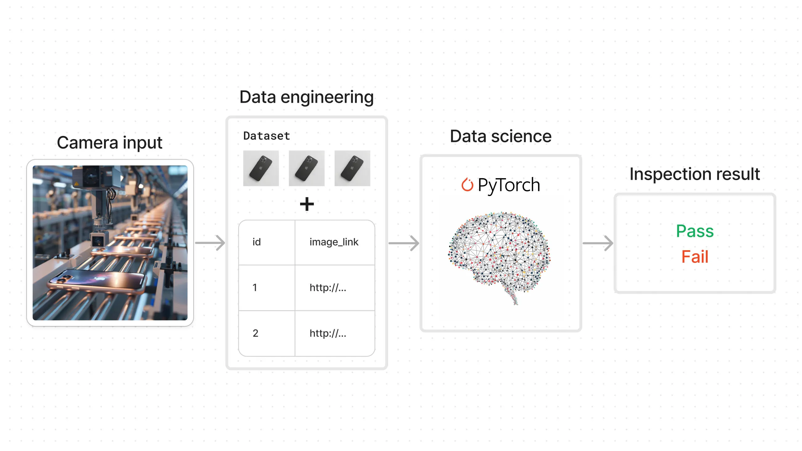
BulletProofGlassCo manufactures the glass cover for the iPhone. In its manufacturing facility, it must determine if there are defects in the glass. Inspecting each unit manually is very expensive, so the company decides to put a camera in its manufacturing line and use an AI model to do the inspection.
The data generated here consists of images from the camera. This data is sent to the data engineering team, which collects them and creates a dataset. This dataset is sent to the data science team, which uses it to build a deep learning model that determines whether the item passes inspection or not.
Conclusion
In this post, we learned what a data pipeline is and how it works. We saw the big picture of how data flows from data sources to data consumers, as well as some example pipelines.
We also got a preview of which tools we’ll be using for each part of the data pipeline.
In the next post, we’ll start to build out the actual data pipeline. We’ll go through the detailed steps of how to set up the tools and connect them together.
Questions and Feedback
If you have any questions or feedback, feel free to join us on Slack and we’ll do our best to help!